Users Guide for ExP to Perform EPIG

Analysis of Gene Expression Data using EPIG (Extracting Patterns and Identifying co-expressed Genes)

Launching ExP

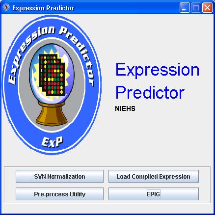
Double click on the EPIG.bat file (dated 10/30/2009). The Expression Predictor dialog box will launch. See below.

Data Format

The gene expression data must be relative change in a fixed/standard tab-delimited text format:

First row: unique array name
Second row: names for replicate groups
First col: probe ID or gene accession

See below:

Convert Intensity Data to Relative Change

If the data is single channel intensity data (Affymetrix or Agilent for example), the data must be converted to relative change using intensity measurements from a baseline experiment, control sample or sham group. Otherwise, skip to the Load Relative Change Data section.

Click the Load Compiled Expression button. The data set will appear in a table. See below.

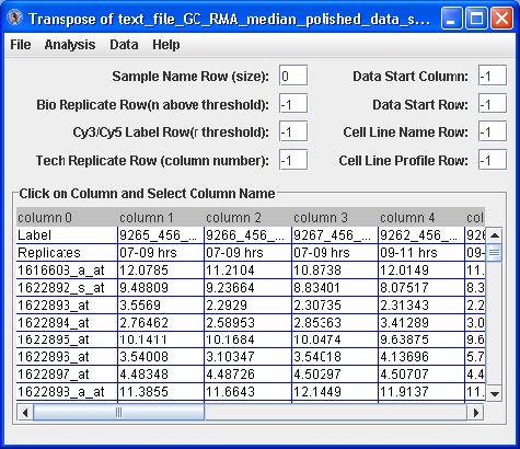
Highlight by clicking the first cell under “column 1”, right click and choose the “Select Data Start Column” option. The “Data Start Column” box value should switch from -1 to 1. Next, highlight by clicking the very first cell (upper most left) with a data value, right click and choose the “Select Data Start Row” option. The “Data Start Row” box value should switch from -1 to 2. Finally, highlight by clicking a cell in the row with the name of one of the replicate samples (i.e. 07-09 hrs in the figure above), right click and choose the “Replicate Row” option. The “Bio Replicate Row” box value should switch from -1 to 1.

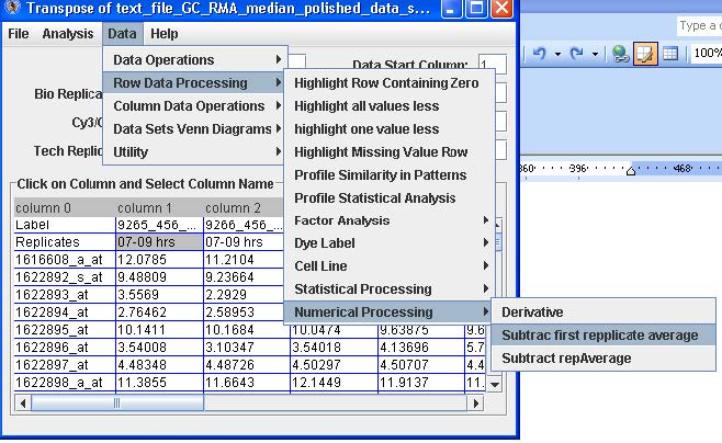
From the menu option select Data → Row Data Processing → Numerical → Processing → Subtract First Replicate Average.

From the Menu option select File → Save Data to save the converted data.

Load Relative Change Data

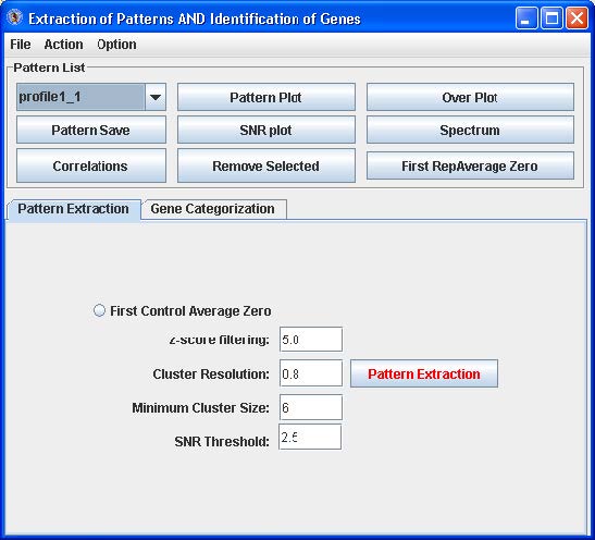
With the data already saved and it is relative change measurements, it can be loaded directly into ExP for EPIG analysis by clicking the EPIG button option on the ExP splash screen. Or, if the converted relative change data is in memory as above, from the Menu option select Analysis → EPIG. The EPIG analysis dialog box will launch. See below.

Cell lines, multiple controls/references/shams adjustment or alignment

You have a case as below.

T1 ctl1 trt11 trt12 trt13… T2 ctl2 trt21 trt22 trt23… T3 ctl3 trt31 trt32 trt33…

At each time point, there is a time matched control. Your input file can be like this –

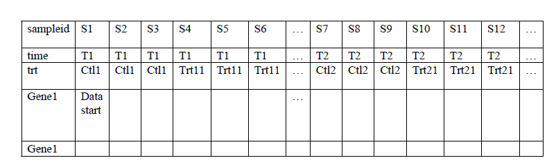
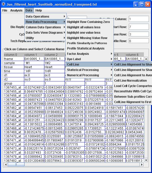
You can select (right mouse button click) time row as cell line name row, and trt row as cell line profile row. Also you select trt row as replicate row.

Then you go to menu Data>Row data processing>cell line>cell line alignment to sham zero. – this will use the ctl as a baseline (average to be zero and all others adjusted accordingly)within its own time point. Then you can save the data if you want and run EPIG.
Another approach is you go to menu Data>Row data processing>Numerical processing>subtract first replicate average – in this case the first control group used as a baseline, then run EPIG

These 2 different approaches will give you different results. Both are interesting. Depending on your focus, you may use one or both results.

EPIG Analysis: Pattern Extraction

The Pattern Extract tab contains an option and fields for parameters that control the extraction of the significant patterns from the gene expression data:

First control Average Zero – click this radio button if the first array data set is a “sham” control or baseline which all the other arrays are compared to
z-score filtering - filters those probes/genes profiles which have one or more data points with z-score larger than the set value
Cluster resolution - correlation threshold to filter those patterns generated with the r-value larger than that to another pattern.
Minimum Cluster size – the number probe/gene profiles to be merged for generating the patterns
SNR Threshold – the threshold for the signal-to-noise for the profiles to be filtered out and thus not used for generating the patterns

Click the “Pattern Extraction” button to generate the patterns. A plot of the extracted patterns will be displayed (see below).

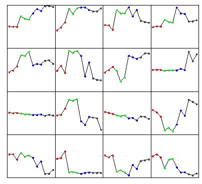
The patterns are arranged in order from the upper-left corner going right. Leave the default settings or go to the menu at the top, Action -> Reset to start over and modify the parameters according to get more or less patterns to be generated. However, from empirical analysis, the default parameters work well. Go to Action -> Rename Pattern Name to name the patterns numerically in the Pattern List drop down.

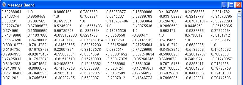
Some patterns will look very similar (i.e. 6 and 10, 9 and 11, 13 and 16). They will likely have a high correlation value. Click the “Correlation” button to see the pairwise correlation values in the Message Board dialog box. See below.

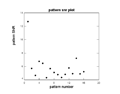
Click the SNR plot button to see a plot of the SRN for each pattern. See below.

The “Message Board” dialog box displays the SNR values, magnitude of change, SNR pvalue, ANOVA test statistic and ANOVA p-value for each pattern. See below.

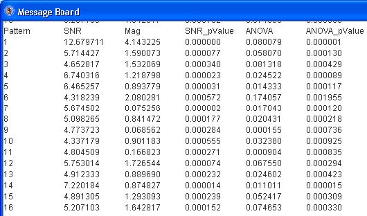
The pattern (of the two similar ones) with the lower SNR (of patterns 13 and 16, pattern 13 has a lower SNR) may be deleted by selecting the pattern from the drop down menu and click the “Remove Selected” button.

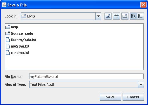
Once you have the number of desired patterns generated, click “Pattern Save” and enter in a name for a file to be generated which will have the patterns and associated parameter values stored in it. See below.

EPIG Analysis: Gene Categorization

Click the Gene Categorization tab (see below).

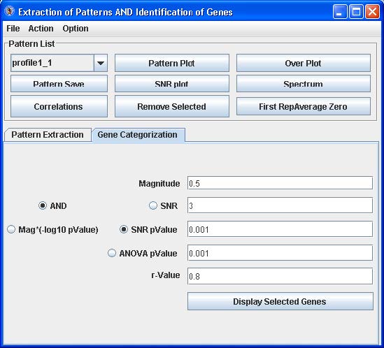
This tab contains parameters that control the binning of probes/genes to the patterns that were generated:

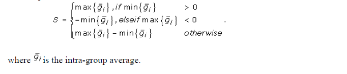
Magnitude (S) – the amount of variation in gene expression within profiles.

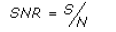
SNR – the signal to noise ratio for the profile

where S is denoted above,

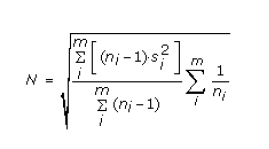
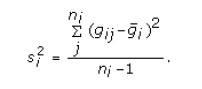
and the sample variance is

SNR p-value – the significance level for the SNR
ANOVA p-value – the significance level for an ANOVA of the profile
r-value – the correlation value for the profile to be similar to the pattern

From empirical analysis, the default parameter settings work well. To adjust the settings, enter a value for Magnitude, click “And”, click the radio button and enter a value for either SNR, SNR p-value or ANOVA p-value, and then enter an r-value. Click Mag*(log10pvlaue) of you want to use the John Zheng modification for categorization of the profiles to the patterns that takes into account both the magnitude of change and the p-value.

Click “Display Selected Genes” to launch up to three dialog boxes as tables with the probe/gene profiles categorized to the patterns, the probe/gene profiles not categorized to particular patterns and the probe/gene profiles categorized to patterns but have low correlation. See below.

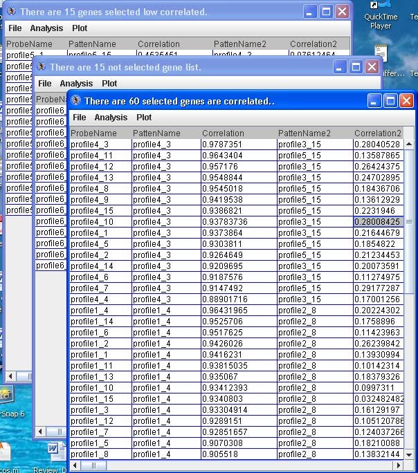
Click “Spectrum” to launch a dialog box as a table with the probe/gene profiles categorized to the particular pattern in the drop down list.

For any of the tables, from the menu go to File -> Save Data or Save in Separate Files to save the probe/gene profiles categorized to patterns. See below.

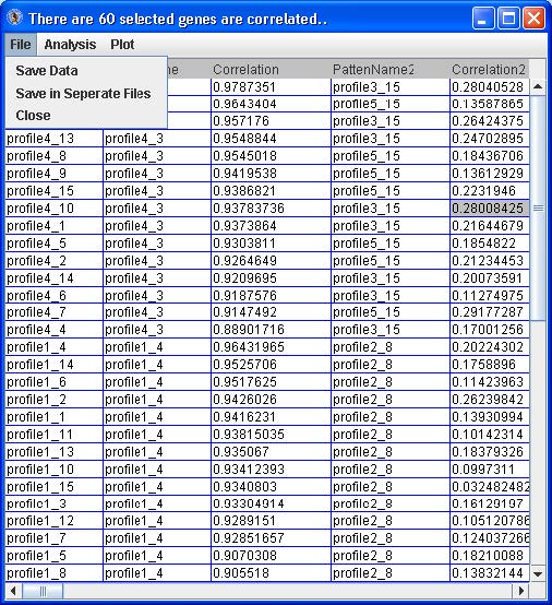
If saving to separate files, the file names will be generated automatically (such as selectedGenesInPattern_2_261.txt) and saved in the working directory for EPIG. The file name contains the pattern number (#2) and the number of probes\genes (n=261) categorized to it.

Reference

Chou JW, Zhou T, Kaufmann WK, Paules RS, Bushel PR. Extracting gene expression patterns and identifying co-expressed genes from microarray data reveals biologically responsive processes. BMC Bioinformatics. 2007 Nov 2;8:427